Showing posts with label BigData. Show all posts

Tuesday, November 21, 2017

1PB in 1U

17 months ago I blogged about 900TB (nearly 1PB) in 1U of rack space for only $60k. There I noted that a 1U server for the new high-density SSDs wasn't commonly available. Well, that has changed. A couple of months ago, Super Micro announced their 32-bay 1U unit for 2.5" drives. With the 32TB SSDs that Samsung announced last year to be available this year, that yields 1PB.

It won't be cheap. Recall that the 900TB 4U for $60k was for spinning drives. Given that the 16TB SSDs go for nearly $12k a pop, the 32TB drive that has been slated for later this year would be at least twice that and likely much more initially. Even at $24k for each 32TB SSD, this 1U of 1PB SSD would set you back $800k.


Saturday, July 30, 2016

900TB, 4U, $60k


The impasse of Peak Hard Drive that I identified two years ago -- that era when 4TB hard drives had been the tops for three years straight -- has been breached, thanks to advances in both hard drives (HDDs) and Solid State Disks (SSDs). 10TB 3.5" HDDs can be ordered from Amazon now for less than $600, and the density of SSDs is skyrocketing as manufacturers promised two years ago. At $10,000, the 2.5" 15TB SSD is indeed dense but at $670/TB, is twice as expensive per terabyte as enterprise 1TB SSDs.
Going forward, Toshiba is predicting 128TB SSDs by 2018 and 40TB HDDs by 2020. As shown in the chart above, SSDs would then firmly breach the long-term exponential growth line in density, while HDDs would merely continue their anemic density growth.

Rack chassis are getting more dense as well. SuperMicro now has a 4U chassis that can hold 90 3.5" HDDs.

Filled with the 10TB HDDs, that would be about $60k for 900TB storage in 4U of rack space. There is no similar solution I've found for 2.5" drives, so using the same chassis for the 15TB SSDs would be $900k for 1.4PB.
But of course that ignores the compute side of the equation. Such ultra-density in a rack would only be suitable for deep-freeze storage. For a Hadoop/Spark application to leverage data locality, a 1U chassis that accommodates 8 2.5" drives and dual processors from SuperMicro would be more appropriate. Populated with the 15TB SSDs, that would be 120TB/1U, or 960TB/8U. If each CPU socket were populated with 22-core Xeons, that would be a total of 352 cores in that 8U. Total cost would be about $750k for that 8U.

Tuesday, February 24, 2015

State of the Stream 2015Q1

The big news this week -- and for the past couple of months, really -- is of course eBay open sourcing theirPulsar real-time analytics framework, which allows SQL queries into a real-time data stream. It's built on top of their Jetstream data streaming framework, also open sourced this month, which, from its list of capabilities seems to be a layer akin to Storm and Spark Streaming, with sinks and sources, Kafka connectivity, and REST interfaces for cluster monitoring.
With all the breathless news items out there about Pulsar, they neglect to mention one important fact: it is GPL, which precludes its use at a lot of organizations.
This is in stark contrast to some other big news this past week: Druid just switched to an Apache license from its use of the GPL.
Streaming is important because as I've previously blogged, every Big Data project eventually becomes a data streaming project, because once insights are found in Big Data, the consumers of those insights request it be re-run with ever more up-to-date data, until eventually they request real-time updates.
I've also previously blogged, over a year ago now, on the comparison of streaming frameworks, especially comparing Storm with Spark Streaming. At the time, I relayed how at the February, 2013 Strata, several speakers spoke of how Trident, the layer that gives Storm exactly once semantics, makes Storm non-performant. I also wrote at that time how Spark Streaming, even though it had exactly-once semantics, lacked things like graceful shutdown and transactions.
Well, there is recent news about about both Spark Streaming and Storm. First, Spark Streaming gained high availability in 1.2.0, released in December, 2014. And although it has exactly once semantics, doing so with Kafka is a bit tricky since Kafka itself does not guarantee exactly once when a node in a Kafka cluster goes down. However, Spark 1.3.0 will have Kafka exactly once semantics. Spark 1.3.0 release candidates are being voted on now, and will probably be released in the first half of March, 2015.
As for performance, a University of Toronto grad student recently benchmarkedStorm vs. Spark Streaming:

"Storm was around 40% faster than Spark, processing tuples of small size (around the size of a tweet). However, as the tuple's size increased, Spark had better performance maintaining the processing times."

Wednesday, December 31, 2014

Using Data To Predict Data Science in 2015


This is the time of the year when pundits make their 2015 predictions. But to make predictions about Data Science, shouldn't one use data? Here are four charts from Google Trends that show trending performance of various data science technologies. Apache Spark really is overtaking Apache Hadoop.


In this R vs. IPython Notebook chart, we should just gather the trends rather than the absolute magnitudes. "R" is notoriously difficult to Google for, and "R Cran" is just one of the many tricks R users employ to Google for information about R. And, sadly, Google Trends has no way to additively combine search trends together (e.g. "R Cran" OR "R Project"). But, we can still see that IPython Notebook is skyrocketing upward while R is sagging.


This is a little hard to read and requires some explaining. The former name for "Apache Storm" was "Twitter Storm" when Twitter first open-sourced Storm onto GitHub in 2011. But "Twitter Storm" has another common usage, which is a "storm of tweets" such as about a celebrity. I'm guessing about half the searches for "Twitter Storm" are for this latter usage.

The takeaway is that Storm got a two-year head start on Spark Streaming and has been chugging away ever since. Part of the reason is that Spark Streaming, despite the surge in popularity of base Spark, had a lot of catching up to do to Storm in terms of graceful handling of errors and graceful shutdown/restart. A lot of that is addressed in the new HA Spark Streaming features introduced in Spark 1.2.0, released a week ago.

But the other interesting trend is that the academic term "complex event processing" is falling away in favor of the more industry-oriented terms "Storm" and "Spark Streaming".


People forget that "Machine Learning" was quite popular back in the dot-com era. And then it started to fade. That is, until Geoffrey Hinton's invention of deep learning in 2006. That seems to have lifted the popularity of machine learning in general. Well, at least we can say there's a correlation.

The other interesting thing is the very recent (within the past month) uptick in interest in DeepMind. Of course there was a barrage of interest in October when the over-hyped headlines blared "mimics human". But I think people only this past month started getting past the hype and started looking at the actual DeepMind paper which is interesting because it shows how they added state to a neural network, and that that is how they achieved "short term memory".

Sunday, November 16, 2014

Parallel vs. Distributed file systems: Time for RAID on Hadoop?


The long-standing wisdom is that RAID is not beneficial for Hadoop data nodes. This wisdom is traced back to the venerable Hadoop: The Definitive Guide, which cites a 2009 Apache forum posting from Yahoo! engineer Runping Qi reporting experimental results showing JBOD to be faster than RAID-0.

The reasons cited in the Hadoop book are:
  • HDFS has redundancy anyway, and
  • RAID-0 slows down the entire array to match the speed of the slowest drive in the array
While the 2009 experimental results are compelling (at least for 2009), these two stated reasons are not.

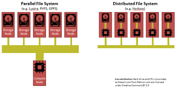
We can look toward "parallel" file systems from the world of High Performance Computing (HPC) for inspiration. The paradigm in HPC is to separate compute from storage, but to have a really fast network, but more importantly to have a "parallel file system". A parallel file system aggregates the bandwidth from many storage nodes to feed a compute node.

While Hadoop was able to achieve its performance through its clever insight of shipping code to data, each CPU in a Hadoop cluster has to suck its data from a single disk through a straw.

The limiting factor for both HPC and Hadoop is the slow transfer rate (1 Gbps) out of a hard drive. HPC addresses this bottleneck by:
  • striping data across nodes,
  • storing data across nodes in a round-robin fashion, rather than the more random approach that Hadoop takes
  • using high-bandwidth links in the cluster (e.g. 40 Gbps Infiniband vs. 1 Gbps or 10 Gbps Ethernet
  • using network DMA (Infiniband) instead of a heavy software stack (Ethernet)
In particular, a 2011 comparison between Lustre and HDFS cited lack of striping in HDFS as a reason for reduced HDFS performance.

There have been a couple chinks in the armor of the "No RAID for HDFS" received wisdom in the past couple of years. The book Pro Apache Hadoop, Second Edition, just published this month, provides one specific exception to the rule:
Some Hadoop systems can drop the replication factor to 2. One example is Hadoop running on the EMC Isilon hardware. The underlying rationale is that the hardware uses RAID 5, which provides a built-in redundancy, enabling a drop in replication factor. Dropping the replication factor has obvious benefits because it enables faster I/O performance (writing 1 replica less).
Another is Hortonworks in 2012, which gives credence to the idea of using RAID-0, but at most only pairs of disks at a time.

It seems that we could have the best of both worlds if each node in a Hadoop cluster had parallel I/O across many disks, such as can be provided by RAID-0. As for the concern that RAID-0 is slowed to the speed of the slowest drive, well, the same is true of PVFS.

So should RAID-0 be used in Hadoop data nodes to speed up I/O to the CPU? Probably not, and here's why. CPUs for the past decade have plateaued on clock speed and have instead been adding cores. And there is a recommendation that there be a 1:1 ratio between "spindles to cores". For the purposes of I/O, multiple hard drives joined in RAID-0 would be considered a single spindle. So one could imagine a single 12-core CPU connected to 12 RAID-0 pairs, for a total of 24 drives. But as core count goes up over the upcoming years, and if dual- and quad-CPU motherboards are considered instead, this scenario becomes the exception.

Sunday, November 9, 2014

Data Locality: HPC vs. Hadoop vs. Spark


Diagram Notes: 1. Yellow documents are map outputs 2. Not shown is that Hadoop spools map outputs to disk before reduce task reads them, whereas Spark keeps the map outputs in RDDs.

The big advance Hadoop brought over classic High Performance Computing (HPC) is data locality. Hadoop brings the compute to the data. (HPC compensates by having faster interconnects such as Infiniband and high-bandwidth storage.)

The big advance Spark brought over Hadoop is storing data in each node's RAM instead of each node's disk. Spark's leveraging of data locality is very similar to that of Hadoop's: namely, computation is assigned to occur where the data resides.

Except Spark 1.2 is set to improve that a bit. In a just published paper, AMP Lab contributor Shivaram Venkataraman et al propose assigning the reduce task to the node that happens to have the largest map output, thus minimizing data movement.

This advance is currently slated for Spark 1.2, in Jira ticket SPARK-2774

There are other advances described in the Venkataraman et al paper, namely, when sampling subsets of data such as BlinkDB does, Spark could greedily take whatever data happens to be present on nodes with available compute, and call that the sample. There is no set Spark release for that feature, which the paper calls KMN.

Four Reasons for Immutable HDFS Archive


Two years ago, when I first joined Michael Walker's Data Science & Business Analytics Meetup, the form asked (and still asks) "What important truth do very few people agree with you on?" My answer was "Data should never be deleted". At the time, I had no idea what Data Science was and had barely been introduced to Big Data, but it was a dictum I lived by, much to the consternation of my bosses over the past two decades when it came time to approve purchases of hard drives.
Well, I may have to update my profile, because it seems more and more people are agreeing with me. As I blogged on the January, 2014 Boulder/Denver Big Data Meetup, the discussion format came to a consensus that all ingested data should be kept intact as-is as an immutable data store, and that processed data should be stored in some kind of data warehouse for the actual analytics. I wrote then that it was good to have that pattern, which was in the making for a couple of years, finally codified as a pattern.
It's even more solidified now. The two most common motivations given are:

1. Bugs

You might discover a bug in your processing code, and so you may need to reprocess all the original data with the corrected code.

2. New Derived Metric

You might discover you need to track clicks per second rather than just clicks per minute. With the original data still around, it becomes possible to resummarize the raw data.

Two Other Reasons

But here are two other reasons, not usually stated when this pattern is presented:

3. New Data Enrichment

Suppose in your summarized data you don't store social security number even though it exists in the original data. Then your company just obtained the services of data provider, and you're now able to get household income based on social security number. Now you can append this data as another column in the analytics database.

4. Reapply Machine Learning to Bigger Data Set

This is perhaps the most important reason of all, due to the The Unreasonable Effectiveness of Data. As more data becomes available over time from the original data streaming source, machine-learned models can be improved.

Sunday, June 8, 2014

SSD to the rescue of Peak Hard Drive?


A couple of months ago, I blogged about Peak Hard Drive, that hard drive capacities were leveling off and how this would impact the footprints of data centers in the era of Big Data. Since then, there have been two major announcements about SSDs that indicate they may come to the rescue:
  1. SanDisk announced 4TB SSD "this year" and 16TB possibly next year. Given that such technologies are typically delayed by one calendar year from their press releases, in the above chart, I've indicated those as becoming available in 2015 and 2016, respectively.
  2. Japanese researches develoepd a technique to improve SSD performance by up to 300%
The 16TB in 2016 is phenomenal and would be four years sooner than the 20TB in 2020 predicted by Seagate. Much more than that, if the 16TB SSD will be in the same form factor as its announced 4TB little brother, then it will be just a 2.5" drive in contrast to the presumed 3.5" form factor for the 20TB Seagate HAMR drive. As you can see in the chart above, the 16TB puts us back on track of the dashed gray line, which represents the storage capacity steady growth we enjoyed from 2004 to 2011.


It is because of the varying form factors that in my blog post two months ago I adopted the novel "Bytes/Liter" metric, which is a volumetric measure in contrast to the more typical "aerial" metric that applies to spinning platters but not to SSDs. (Actually I changed the metric from log10(KB/Liter) from two months ago to log10(Bytes/Liter) now, reasoning that Bytes is a more fundamental unit than KB, that it eliminates the KB vs. KiB ambiguity, and that it makes the chart above easier to read where you can just pick out the MB, GB, TB, PB by factors of 3 of the exponent of 10.) This volumetric metric can handle everything from the 5.25" full-height hard drives of the 1980's to the varying heights of 2.5" hard drives and allow us to linearly extrapolate on the logarithm chart above.

The direct overlay of the SSD line over the HDD line for the years 1999-2014 came as a complete shock to me. SSDs and HDDs have vastly different performance, form factor, price and performance characterstics. Yet when it comes to this novel metric of volumetric density, they've been identical for the past 15 years!


Photo from tomshardware.com comparing 9.5mm height 2.5" drive to 15mm

Now, the announced 4TB 2.5" SSD and presumably also the 16TB SSD are not of the typical notebook hard drive form factor. The typical notebook hard drive is 9.5mm tall, whereas these high-capacity SSDs are 15mm tall. They're intended for data center use, such as in the 2U rack below.

The configuration in the 2U chassis above is typical for 2.5" drives: just 24 drives, because they are all accessible from the front panel. I'm not aware of any high-density solutions for 2.5" drives such as those that exist for 3.5" drives, such as the one below that puts 45 drives into 4U.

In time, there should be some higher density rackmount solutions for 2.5" drives appearing, but for now, today's available solutions don't take full advantage of the compactness of 2.5" SSDs portrayed in the above chart, which measures volumtric density of the drive units themselves and not the chassis in which they reside.
Also not clear is whether the 16TB SSD will be MLC or TLC. The 4TB drive is MLC, which means two bits per cell. If the 16TB drive is TLC, then three bits are stored in each cell (eight different voltage levels detected per cell), which can reduce lifespan by a factor of 3 and for that reason are often not considered for enterprise data center use.

For the moment, we're stuck at the inflection point in the above chart at 2014, wondering which dotted line data centers will be able to take in the future.


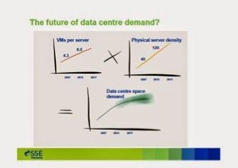
Due to a combination of increased use of VMs in data centers and increased physical server density, projections were that we had reached peak physical square footage for data centers: that no more data centers would have to be built, ever (aside from technology improvements such as cooling and energy efficiency). The slide above is from SSE. My blog on Peak Hard Drive threatened to blow that away and require more data centers to be built due to plateauing hard drive density combined with exploding Big Data use. But now with the two SSD announcements, we might be -- just maybe -- back on track for no more net data center square footage.

Sunday, May 4, 2014

Peak Hard Drive

This past week, Seagate finally announced a 6TB hard drive, which is three years after their 4TB hard drive. Of course, Hitachi announced their hermetically-sealed helium 6TB hard drives in November, 2013, but only to OEM and cloud customers, not for retail sale.

Hard drive capacities are slowing down as shown in the chart below. To account for the shrinking form factors in the earlier part of the history, and to account for exponential growth, I've scaled the vertical axis to be the logarithm of kilobytes (1000 bytes) per liter.


This three year drought on hard drive capacity increases is represented by the plateau between the last two blue dots in the graph, representing 2011 and 2014. The red line extension to 2020 is based on Seagate's prediction that by then they will have 20TB drives using HAMR technology, which uses a combination of laser and magnetism.

However, if the trendline from 2004-2011 had continued, by linear extrapolation on this log scale, hard drives would have been 600TB by 2020.

This is not good news for users of Big Data. Data sizes (and variety and number of sources) are continuing to grow, but hard drive sizes are leveling off. Horizontal scaling is no longer going to be an option; the days of the monolithic RDBMS are numbered. Worse, data center sizes and energy consumption will increase proportional to growth in data size rather than be tempered by advances in hard drive capacities as we had become accustomed to.

We haven't reached an absolute peak in hard drive capacity, so the term "peak hard drive" is an exaggeration in absolute terms, but relative to corporate data set sizes, I'm guessing we did reach peak hard drive a couple of years ago.

Saturday, December 28, 2013

Real-time Data Science

Looking back on 2013, the world of Hadoop emerged from the era of batch processing and into streaming processing. In the contextg of "crisp and actionable," actionable often comes with an expiration date. If you don't take action soon enough, it's too late.

As I learned at the February 2013 Strata conference, Electronic Arts instrumented their online games to continuously stream data into their Big Data system. And because much of their revenue now comes from in-game purchases (in games that are often free to play), they need to know immediately if, e.g., in-game purchases suddenly drop off for whatever reason. They need to take action immediately, not next week.

Here I look at four streaming technologies, and then conclude with some pointers to general streaming computation techniques.

Part of the Berkeley Data Analytics Stack, Spark Streaming is a layer on top of Spark. Spark is a distributed, redundant RAM-based data storage and computation system that was accepted as an Apache Incubator project in 2013. Whereas Hadoop distributes data across the hard drives in a cluster of computers, Spark distributes data across the RAMs in a cluster of computers.

Spark Streaming breaks incoming stream into batches of, for example, 2-second batches or 10-second batches, or however long you set the batch window to be. One criticism of Spark Streaming is that it is not "true real time" since it is up to a batch window size behind. Another limitation is that all processing for that batch must complete before the next batch comes in; otherwise, the behavior is undefined. That can leave a lot of compute capacity unused if the system is tuned to handle the worst-case batch, but normal-size batches leave the processors idle for much of the batch time window.


Storm, another Apache project originally from Twitter, is the other big name in streaming. Its biggest and most well-known shortcoming is that it doesn't guarantee that it won't duplicate events. It guarantees each event will delivered at minimum once. Since this can wreak havoc with real-time metric computation, an optional layer called Trident can de-dupe, but at a high performance penalty.

Storm has a great advantage over Spark Streaming in that it has an "ack" system built-in. If processing an event throws an exception or otherwise fails to "ack" its parent in the directed acyclic graph (DAG) of event flow processing, the event can be saved by the parent for later processing when the problem has been fixed.
Storm also has a web-based admin GUI for starting/stopping/monitoring running DAGs.

Since I don't have any first-hand experience with S4, I have to rely on others' evaluations. At a presentation by Ted Dunning of MapR, he indicated that S4 was designed for topologies and situations that are more complex than usually encountered in the real world. A Yahoo! researcher blogged an excellent comparison between S4 and Storm, and boils it down to guaranteed delivery (Storm) vs. state recovery in case of fault (S4).

Druid is different than the rest in that it's more than just streaming; it also provides a data store and querying system. It's an all-in-one solution whereas the others are usually married to Hadoop.

Druid breaks the storage into two parts, one for real-time (typically 30 minutes worth of data), and the other for permanent "deep storage". A single querying facade can query both stores transparently.

The bad news is that the querying is currently limited. With no SQL, queries must be formed using a stilted JSON syntax, and the ability to create complex queries is limited.
But querying is fast. In fact, it's Druid's hallmark. In response to the common problem of cubing data with high dimensionality, the Druid folks decided instead to just be able to query really fast by storing the data in a distributed RAM-based cluster. With fast querying, there's no need to pre-compute and pre-aggregate.

LinkedIn contributed Samza to Apache in September, 2013. It's new and I haven't tried it yet, but it appears to integrate Kafka and YARN more deeply than the others, and it maintains state similar to how Spark Streaming allows with its RDDs (resilient distributed dataset) and its updateStateByKey() method.

While all the others are for self-hosted infrastructure, Amazon Kinesis is strictly for the could. Again, since I haven't used it myself, I rely on another blogger who informs that Kinesis is restricted to a single procedure, and so isn't suited for complex processing. There is also no rollback capability.

Stream Computation Techniques

It's evident fairly quickly that the mean can be computed in an incremental manner. If mn is the mean of x1 ... xn, then mn+1 = (n*mn + xn+1)/(n+1).

Much less obvious is that it's possible to calculate the standard deviation incrementally. Donald Knuth credits a 1962 paper by Welford with a clever technique.

Even more clever is calculating cardinality incrementally, i.e. the number of distinct items in a set, i.e. SELECT COUNT DISTINCT(*) -- and doing so without having to keep the entire dataset in memory. The trick is to use a hash function that uniformly distributes to the range [0.0,1.0) and then keep track of the most number of leading zeroes. E.g. if the set as 100 items, probabilistically we would expect the smallest hash value to end up being around 0.01, or one leading zero. For a set of 1000 items, some hash values by chance would probably end up being less than that, and the smallest overall would probably end up being around 0.001, or two leading zeroes.

Finally, classic machine learning algorithms such as K-means and decision tree construction have been adapted to incremental versions for streaming data. Joao Gama, a Portuguese professor, has assembled them into an excellent book:

Applications

Basic metrics permit real-time monitoring for:

  • Fraud detection
  • Fault detection
  • Capacity overload detection

Streaming machine learning adds:

  • Intelligent automated adjustment of thresholds to the above
  • Ability to detect opportunities, not just problems. E.g. product affinity of noticing products long-time product A and brand-new product B could alert management to craft a marketing campaign for product B to those who have bought A in the past.

Conclusion

While "real-time data science" doesn't mean taking conventional, manual, deep data exploration and analysis and applying it to real-time data, what it does mean for data scientists is that they are increasingly feeling the pressure to have some results automated and real-time, and data scientists need to be comfortable with these streaming technologies and algorithms.

Wednesday, April 24, 2013

Presentation on Spark

Last night I gave a presentation on Spark, the exciting replacement for Hadoop's Map/Reduce that's come out of Berkeley and not tied to any particular distribution of Hadoop. Slides and video are below (video is cued to start at my part at 12:25, and it goes for about 35 minutes).

Thursday, March 21, 2013

Kafka tips

Three tips on using Kafka:
  1. Use buffer.remaining() instead of buffer.array().

    Kafka's message.payload() returns a ByteBuffer, and if you need access to the raw bytes, it's tempting to just call message.payload().array(), but that would be the wrong thing to do. That returns the backing array to the ByteBuffer, which may (and in the case of Kafka usually is) larger than the data it represents, with offsets and limits maintained by ByteBuffer.

    Sadly, there is no single-line solution. Below is the most concise way to get the raw bytes out of a Kafka message and into a plain vanilla byte[] array.

    ByteBuffer buffer = message.payload();
    byte[] bytes = new byte[buffer.remaining()];
    buffer.get(bytes);
    
  2. If sending Avro over Kafka, then serialize using EncoderFactory instead of DataFileWriter with ByteArrayOutputStream, for two reasons:

    • DataFileWriter writes out an entire Avro file, complete with schema. Sending the schema with every Kafka message is a waste.
    • If you plan to consume Kafka messages with Camus, then you need to use EncoderFactory because Camus uses DecoderFactory.
  3. encoder.flush()

    If sending Avro over Kafka and using EncoderFactory, then don't forget to call encoder.flush() after writing, as in this Avro Hello World example.

Friday, March 1, 2013

Strata 2013 Santa Clara trip report

Strata, the O'Reilly conference on Big Data, just wrapped up Feb 26-28, 2013 in Santa Clara. The story of 2013 is we're entering the post-Hadoop -- read all the juicy details about Big Data, Data Science, and Visualization in my daily trip reports:

Strata Trip Report: Days 0 & 1
Strata Trip Report: Day 2
Strata Trip Report: Day 3

Friday, December 21, 2012

Javascript Dagre & D3 to visualize Big Data dataflows

Big Data projects often involve a lot of stovepipe processing, and visualizing data flows is a powerful way to convey data provenance to the end user, and even allow control of the involved processes.

There are a number of tools available to visualize data flows, but most suffer from some limitation. Some allow labeling of only nodes, but not edges. Some do not have a provision for the node label to be inside of the node. Most use general-purpose graph layout algorithms such as "gravity", whereas dataflow diagrams have distinct start nodes and end nodes and are better represented mostly orthoganlly either top-down or left-right. (The well-known dataflow language G from LabVIEW is left-right, but top-down is better suited for web browsers.)  Graphviz can generate a nice top-down layout, but for the web can only at this time produce static images (albeit dynamically), with no mouseovers to facilitate drill-downs into processes or data stores.

Dagre, a Javascript library built on top of the D3.js visualization toolkit, is very well-suited to visualizing Big Data data flows. Below is an example (contrived, but illustrates the idea):


Dagre generated the above from the succinct input below:

digraph {
    A [label="Apache"];
    B [label="fetchlog.sh"]
    C [label="parseaccesslogs.pig"];
    D [label="parseerrorlogs.pig"];
    E [label="PageViewsPer503"];
    A -> B [label="access_log"];
    A -> B [label="error_log"];
    B -> C [label="/logs/access_log_$DATE.txt"]
    B -> D [label="/logs/error_log_$DATE.txt"]
    C -> E [label="MySQL:VISITORS"];
    D -> E [label="MySQL:ERRORS"];
}

You can paste it into Dagre's live demo yourself, and you can see that mouseover highlighting is possible, meaning it is possible to hook it to do drill-downs.